number_ones[1] "John" "Robert" "James" "Michael" "David" "Jacob" "Noah"
[8] "Liam" Apply your knowledge of dplyr to do the following two challenges.
How many distinct boys names achieved a rank of Number 1 in any year?
How many distinct girls names achieved a rank of Number 1 in any year?
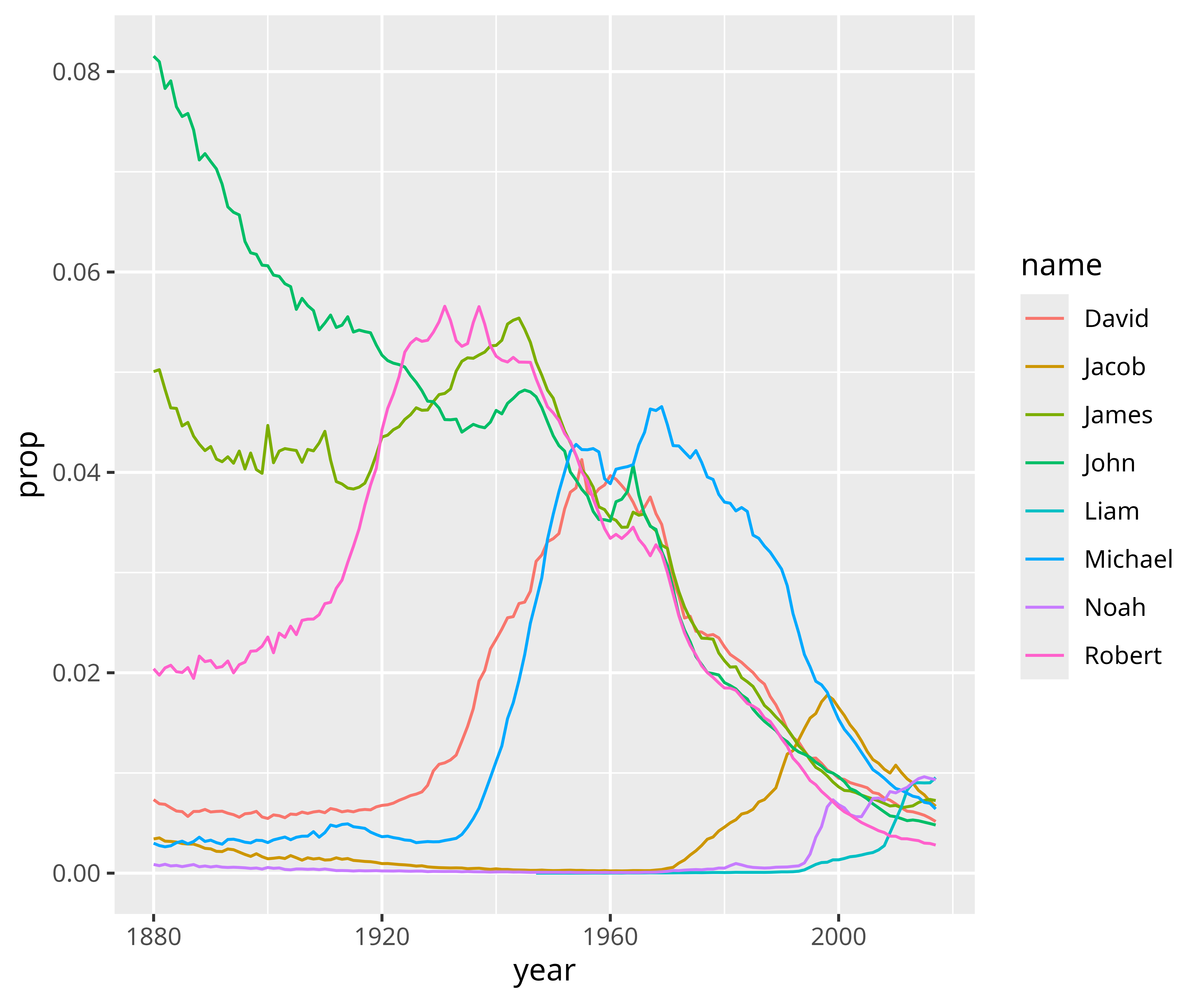
number_ones is a vector of every boys name to achieve a rank of one.
Use number_ones with babynames to recreate the plot below, which shows the popularity over time for every name in number_ones.
babynames |>
  filter(name %in% number_ones, sex == "M") |>
  ggplot() +
    geom_line(aes(x = year, y = prop, color = name))
Which gender uses more names?
In the chunk below, calculate and then plot the number of distinct names used each year for boys and girls. Place year on the x axis, the number of distinct names on they y axis and color the lines by sex.
Let’s make sure that we’re not confounding our search with the total number of boys and girls born each year. With the chunk below, calculate and then plot over time the total number of boys and girls by year. Is the relative number of boys and girls constant?
Hmm. Sometimes there are more girls and sometimes more boys. In addition, the entire population has been grown over time. Let’s account for this with a new metric: the average number of children per name.
If girls have a smaller number of children per name, that would imply that they use more names overall (and vice versa).
In the chunk below, calculate and plot the average number of children per name by year and sex over time. How do you interpret the results?
Good job! In recent years, there are fewer girls (on average) given any particular name than boys. This suggests that there is more variety in girls names than boys names once you account for population. Interestingly, the number of children per name has gone down steeply for each gender since the 1960s, even though the total population has continued to increase. This suggests that there is a greater variety of names today than in the past.
Congratulations! You can use {dplyr}’s grammar of data manipulation to access any data associated with a table—even if that data is not currently displayed by the table.
In other words, you now know how to look at data in R, as well as how to access specific values, calculate summary statistics, and compute new variables. When you combine this with the visualization skills that you learned in Visualization Basics, you have everything that you need to begin exploring data in R.
The next tutorial will teach you the last of three basic skills for working with R: